9.3 Representing Relations Apr 23, 2018 Shawn Math 240 No comments yet Math 541 – 4/20 Apr 22, 2018 Shawn Math 541 No comments yet Math 521 – 4/20 Apr 22, 2018 Shawn Math 521 No comments yet Math 521 – 4/18 Apr 22, 2018 Shawn Math 521 No comments yet Math 521 – 4/16 Apr 22, 2018 Shawn Math 521 No comments yet 1 … 14 15 16 17 18 … 60
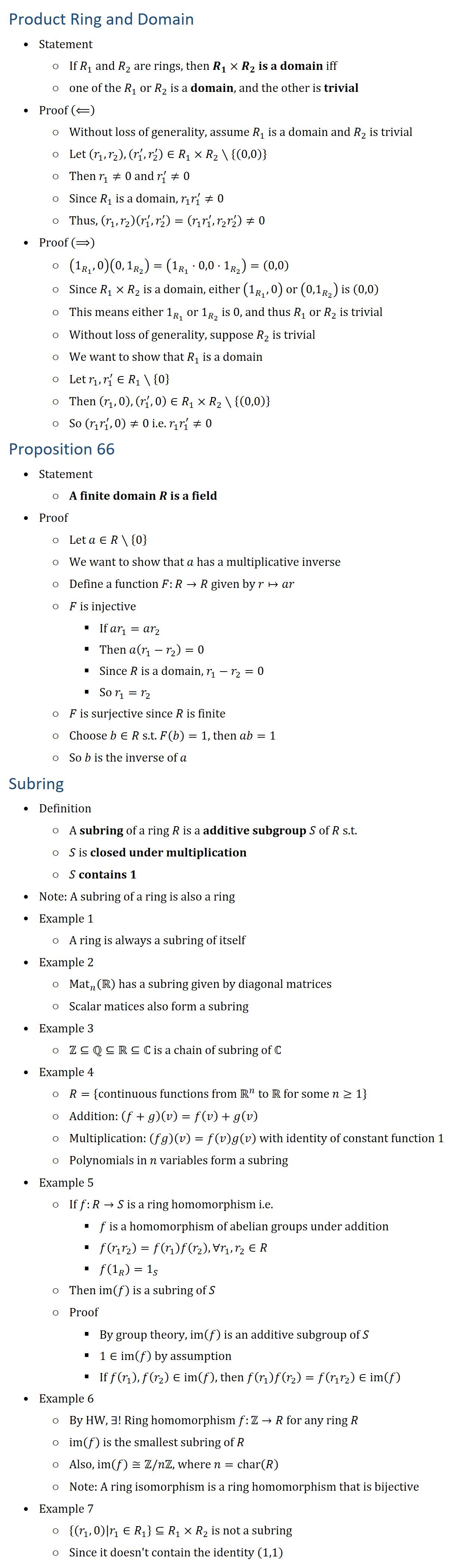
![Representing Relations Using Matrices • A relation between finite sets can be represented using a zero-one matrix. • Suppose R is a relation from A={a_1,a_2,…,a_m } to B={b_1,b_2,…,b_n } ○ The elements of the two sets can be listed in any arbitrary order ○ When A=B, we use the same ordering. • The relation R is represented by the matrix ○ M_R = [m_ij], where ○ m_ij={■8(1&if (a_i,b_j )∈R@0&if (a_i,b_j )∉R)┤ • The matrix representing R has ○ a 1 as its (i,j) entry when a_i is related to b_j ○ a 0 if a_i is not related to b_j. Examples of Representing Relations Using Matrices • Example 1 ○ Suppose that A = {1,2,3} and B = {1,2} ○ Let R be the relation from A to B containing (a,b) if a b. ○ What is the matrix representing R (with increasing numerical order) • Solution ○ Because R={(2,1), (3,1),(3,2)}, the matrix is ○ M_R=[■8(0&0@1&0@1&1)] • Example 2 ○ Let A={a_1,a_2, a_3} and B={b_1,b_2, b_3,b_4, b_5}. ○ Which ordered pairs are in the relation R represented by the matrix ○ M_R=[■8(0&1&0&0&0@1&0&1&1&0@1&0&1&0&1)] • Solution ○ Because R consists of those ordered pairs (a_i,b_j) with m_ij = 1 ○ R={(a_1, b_2), (a_2, b_1),(a_2, b_3), (a_2, b_4),(a_3, b_1), {(a_3, b_3 ), (a_3, b_5 )} Matrices of Relations on Sets • If R is a reflexive relation, all the elements on the main diagonal of M_R are equal to 1 • R is a symmetric relation, if and only if m_ij = 1 whenever m_ji = 1 • R is an antisymmetric relation, if and only if m_ij = 0 or m_ji = 0 when i≠j Example of a Relation on a Set • Example 3: Suppose that the relation R on a set is represented by the matrix ○ M_R=[■8(1&1&0@1&1&1@0&1&1)] • Is R reflexive, symmetric, and/or antisymmetric? • Because all the diagonal elements are equal to 1, R is reflexive • Because M_R is symmetric, R is symmetric • R not antisymmetric because both m_1,2 and m_2,1 are 1 Representing Relations Using Digraphs Definition ○ A directed graph, or digraph, consists of a set V of vertices (or nodes) together with a set E of ordered pairs of elements of V called edges (or arcs). ○ The vertex a is called the initial vertex of the edge (a,b) ○ The vertex b is called the terminal vertex of this edge. ○ An edge of the form (a,a) is called a loop. Example 1 ○ A drawing of the directed graph with vertices a, b, c, and d ○ and edges (a, b), (a, d), (b, b), (b, d), (c, a), (c, b), and (d, b) is shown here. Example 2 ○ What are the ordered pairs in the relation represented by this directed graph? § ○ The ordered pairs in the relation are ○ (1, 3), (1, 4), (2, 1), (2, 2), (2, 3), (3, 1), (3, 3), (4, 1), (4, 3) Determining which Properties a Relation has from its Digraph • Reflexivity: A loop must be present at all vertices in the graph. • Symmetry: If (x,y) is an edge, then so is (y,x). • Antisymmetry: If (x,y) with x≠y is an edge, then (y,x) is not an edge. • Transitivity: If (x,y) and (y,z) are edges, then so is (x,z) Determining which Properties a Relation has from its Digraph • Example 1 ○ Reflexive? No, not every vertex has a loop ○ Symmetric? Yes (trivially), there is no edge from one vertex to another ○ Antisymmetric? Yes (trivially), there is no edge from one vertex to another ○ Transitive? Yes, (trivially) since there is no edge from one vertex to another • Example 2 ○ Reflexive? No, there are no loops ○ Symmetric? No, there is an edge from a to b, but not from b to a ○ Antisymmetric? No, there is an edge from d to b and b to d ○ Transitive? No, there are edges from a to c and from c to b, but there is no edge from a to d • Example 3 ○ Reflexive? No, there are no loops ○ Symmetric? No, for example, there is no edge from c to a ○ Antisymmetric? Yes, whenever there is an edge from one vertex to another, there is not one going back ○ Transitive? No, there is no edge from a to b • Example 4 ○ Reflexive? No, there are no loops ○ Symmetric? No, for example, there is no edge from d to a ○ Antisymmetric? Yes, whenever there is an edge from one vertex to another, there is not one going back ○ Transitive? Yes (trivially), there are no two edges where the first edge ends at the vertex where the second edge begins Closures • Definition ○ The closure of a relation R on A with respect to property P ○ is the least relation on A that contains R and has property P • Note ○ Least relation R^′ on A s.t. ○ R⊆R′ ○ R′ has property P ○ If S is a relation that safisfies the condition above, then R^′⊆S • Example ○ The reflexive closure of R is just R∪{(a,a)│a,∈A} ○ The symmetric closure of R is R∪R^(−1) ○ The transitive closure of R is R∪R^2∪R^3∪… Path in Directed Graphs • Definition ○ A path from a to b is a directed graph G is a sequence of edges ○ (a=x_0,x_1 ),(x_1,x_2 ),…,(x_(n−1),x_n=b) where n 0 ○ We denote the path by x_0,x_1,…,x_n say that the path has length n • Theorem ○ Let R be a relation on a set A ○ There is a path of length n from a to b if and only if (a,b) is an element of R^n The Connectivity Relation • Definition ○ Let R be a relation on A ○ The connectivity relation R^∗ cibsusts if all elements (a,b) s.t. ○ There is a path from a to b in R ○ In other words, R^∗ is the union of R,R^2,R^3,… ○ R^∗=⋃24_(i=1)^∞▒R^((i) ) • Example 1 ○ Let R be the relation between US state such that (a,b) is in R if a and b share a border. What is R^∗? ○ All pairs of states except Alaska and Hawaii • Example 2 ○ Let R be the relation between integers s.t. (a,b) is in R if b=a+1 ○ What is R^2, R^n, R^∗ ○ R^2={(a,b)│b=a+2} ○ R^n={(a,b)│b=a+n} ○ R^∗={(a,b)│a b} • Transitive closure ○ The connectivity relation R^∗ is exactly the transitive closure of R ○ We need to show that R is a subset of R^∗, R^∗ is transitive and least with that property. ○ The first two are easy ○ Let S be a transitive relation containing R ○ By induction we show that S contains R^n for every n Computing The Connectivity Relation • Theorem ○ Let R be a relation on A and let n be the number of elements in A. ○ The connectivity relation R^∗ is the union of R,R^2,…,R^n • Proof ○ Let (a,b) be the element of R^∗ ○ Let a_0=x_0,x_1,…,x_m=b be the shortest path witnessing this. ○ If m n, then two of the vertices among x_1,…,x_m must be the same, say x_i=x_j ○ But then we can find a shorter path x_0,x_1,…,x_i=x_j,x_(j+1),x_n • Corollary ○ M_(R^∗ )=M_R∨M_R^[2] ∨…∨M_R^[n] • Example ○ Compute M_(R^∗ ) for the relation R={(a,b),(b,c),(c,d),(d,b)} ○ M_R=[■8(0&1&0&0@0&0&1&0@0&0&0&1@0&1&0&0)] ○ M_R^[2] =[■8(0&1&0&0@0&0&1&0@0&0&0&1@0&1&0&0)]⨀[■8(0&1&0&0@0&0&1&0@0&0&0&1@0&1&0&0)]=[■8(0&0&1&0@0&0&0&1@0&1&0&0@0&0&1&0)] ○ Similarly, compute M_R^[3] ,M_R^[4] ○ Then M_(R^∗ )=M_R∨M_R^[2] ∨M_R^[3] ∨M_R^[4]](https://shawnzhong.com/wp-content/uploads/2018/04/img_5added4674c91.png)

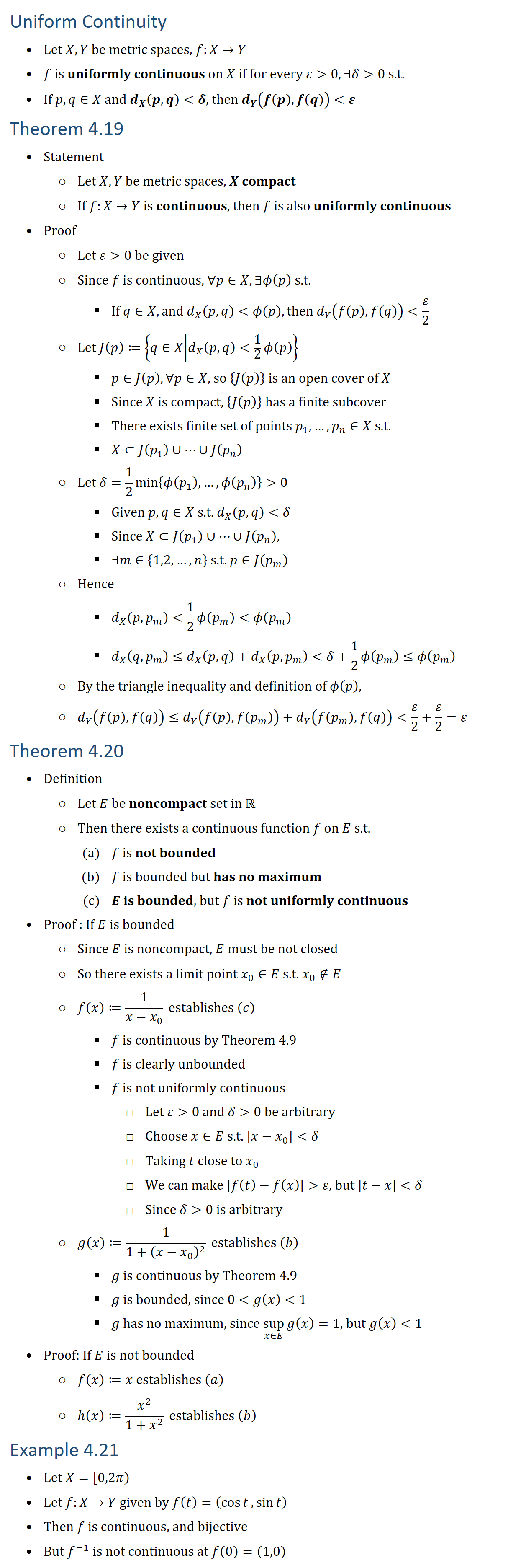
![Continuous • Definition ○ Suppose X,Y are metric spaces, E⊂X, p∈E, and f:E→Y ○ f is continuous at p if for every ε 0, there exists δ 0 s.t. ○ If x∈E,d_X (x,p) δ, then d_Y (f(x),f(p)) ε ○ If f is continuous at every point p∈E, then f is continuous on E • Note ○ f must be defined at p to be continous at p (as opposed to limit) ○ If p is an isolated point of E ○ Then every function f whose domain is E is continous at p Theorem 4.6 • In the context of Definition 4.5, if p is also a limit point of E, then • f is continious at p if and only if (lim)_(x→p)f(x)=f(p) Theorem 4.7 • Statement ○ Suppose X,Y,Z are metric spaces, E⊂X,f:E→Y, g:f(E)→Z, and ○ h:E→Z defined by h(x)=g(f(x)),∀x∈E ○ If f is continuous at p∈E, and g is continuous at f(p) ○ Then h is continuous at p • Note: h is called the composition of f and g and is called g∘f • Proof ○ Let ε 0 be given ○ Since g is continuous at f(p),∃η 0 s.t. § If y∈f(E) and d_Y (y,f(p)) η, then d_Z (g(y),g(f(p))) ε ○ Since f is continuous at p, ∃δ 0 s.t. § If x∈E and d_X (x,p) δ, then d_Y (f(x),f(p)) η ○ Consequently, if d_X (x,p) δ, and x∈E, then § d_Z (g(f(x)),g(f(p)))=d_Z (hx),hp)) ε ○ So, h is continuous at p by definition Theorem 4.8 • Statement ○ Given metric spaces X,Y ○ f:X→Y is continuous if and only if ○ f^(−1) (V) is open in X for every open set V⊂Y • Proof (⟹) ○ Suppose f is continuous on X, and V⊂Y is open ○ We want to show all points of f^(−1) (V) are interior points ○ Suppose p∈X, and f(p)∈V, then p∈f^(−1) (V) ○ V is open, so ∃ε 0 s.t. y∈V if d_Y (f(p),y) ε ○ Since f is continuous at p, ∃δ 0 s.t. § If d_X (x,p) δ, then d_Y (f(x),f(p)) ε ○ So x∈f^(−1) (V) if d_X (x,p) δ ○ This shows that p is an interior point of f^(−1) (V) ○ Therefore f^(−1) (V) is open in X • Proof (⟸) ○ Suppose f^(−1) (V) is open in X for every open set V⊂Y ○ Fix p∈X, ε 0 ○ Let V≔{y∈Y│d_Y (y,f(p)) ε } ○ V is open, so f^(−1) (V) is also open ○ Thus, ∃δ 0 s.t. if d_X (p,x) δ, then x∈f^(−1) (V) ○ But if x∈f^(−1) (V), then f(x)∈V so d_Y (f(x),f(p)) ε ○ So, f:X→Y is continuous at p ○ Since p∈X was arbitrary, f is continuous on X • Corollary ○ Given metric spaces X,Y ○ f:X→Y is continuous on X if and only if ○ f^(−1) (V) is closed in X for every closed set V in Y • Proof ○ A set is closed if and only if its complement is open ○ Also, f^(−1) (E^c )=[f^(−1) (E)]^c, for every E⊂Y](https://shawnzhong.com/wp-content/uploads/2018/04/img_5add053c62b0b.png)